3.1 Modeling Linear Relationships with Algebra

Learning Objectives

Upon completion of this section, you should be able to

Identify elements in a linear model of the form $y = m x + b$
Create a linear model with algebra between two quantitative variables
Graph a linear model
Solve application problems using a linear model created with algebra

Linear Models

Two variables are in linear relationship if we can describe how they change together by adding or subtracting a fixed constant for each unit increase in one variable. For example the cost for hiring a plumber may start with a $75 fee for coming to your house plus an hourly rate of $60. The two variable here are the total cost for the job and the number of hours needed to complete it. For each one hour increase to complete the job we would see an increase of $60 to the total cost.

What you will work on in this section is how to write an algebraic model to describe that relationship between two variables in applications. We will start with the general equation of a line in slope-intercept form.

Linear Model

A linear model (equation) has the form $y = m x + b$ .

b is the $y - intercept$ of the graph and indicates the point $(0, b)$ at which the graph crosses the $y - axis$ .
m is the slope of the line (also called the rate of change) and indicates the vertical displacement (rise) and horizontal displacement (run) between each successive pair of points. The formula for slope between two points $(x_{1}, y_{1}) and (x_{2}, y_{2})$ is: $m = \frac{change in output (rise)}{change in input (run)} = \frac{Δ y}{Δ x} = \frac{y_{2} - y_{1}}{x_{2} - x_{1}}$

We call this form of a linear equation the slope-intercept form as it gives the information about the slope, m, and y-intercept, b.

Example 1

Which of the following represent a linear model. If it is a linear model identify the slope m and intercept b.

$y = 10 x + 20$
$y = x^{2} + 4$
$y = 5 + 2^{x}$
$y = 5 + 2 x$
$y = 100 - 45 x$

Solutions

This is a linear model. Slope is 10 and the y-intercept is 20.
This is not a linear model as we are squaring the x term in the equation.
This is not a linear as the second term in the equation $2^{x}$ has x in the exponent.
This is a linear model. We can rewrite it as $y = 2 x + 5$ . The slope is 2 and the y-intercept is 5.
This is a linear model. We can rewrite it as $y = - 45 x + 100$ . The slope is -45 and has a y-intercept of 100.

Before we look at applications lets review how to create a linear model for given sets of points and identify the key elements of slope and intercept.

Example 2

Find a linear model that goes through the points $(4, 1) and (5, 3)$

Solution

When given two points you start with the slope formula to find m:

\begin{array}{l} m = \frac{(3 - 1)}{(5 - 4)} \\ m = \frac{2}{1} \\ m = 2 \end{array}

Now we were not given the y-intercept directly, so we will first update the linear model with our information about the slope: $y = 2 x + b$

Now to find b we can use either of the two given points to put into the equation and solve. We will use $\begin{array}{l} (4, 1) \end{array}$ in the work below.

\begin{array}{l} y = 2 x + b \\ 1 = 2 (4) + b, where y = 1 and x = 4 \\ 1 = 8 + b \\ 1 - 8 = b \\ - 7 = b \end{array}

Putting our value in for b we get the linear model is: $y = 2 x - 7$

Try it Now 1

Find the equation of a line that goes through the points $(- 4, 5) and (2, 3)$ .

Hint 1

Start with the slope of the line. The slope formula is below. After finding the slope you can use either point given and the slope in the equation to find the y-intercept value b.

m = \frac{change in output (rise)}{change in input (run)} = \frac{Δ y}{Δ x} = \frac{y_{2} - y_{1}}{x_{2} - x_{1}}

Hint 2

The slope is:

m = \frac{(3 - 5)}{2 - (- 4)} = - \frac{2}{(2 + 4)} = - \frac{2}{6} = - \frac{1}{3}

Answer

First find the slope of the line: $m = \frac{(3 - 5)}{2 - (- 4)} = - \frac{2}{(2 + 4)} = - \frac{2}{6} = - \frac{1}{3}$

Next we add the value of the slope to the equation of the line: $y = - \frac{1}{3} x + b$

Use either point given in the equation to find b:

\begin{array}{l} 3 = - \frac{1}{3} (2) + b \\ 3 = - \frac{2}{3} + b \\ 3 + \frac{2}{3} = b \\ \frac{9}{3} + \frac{2}{3} = b \\ \frac{11}{3} = b \end{array}

The equaiton of the line through $(- 4, 5) and (2, 3)$ is $y = - \frac{1}{3} x + \frac{11}{3}$

Graph a Linear Model

We will start from a linear model and graph the line with two different strategies (plot by points and plot using information about the line from the given information of slope and intercept).

Graphing a linear model by plotting points

To find points on a graph for any model, we can choose input values and evaluate the model at these input values to find the corresponding output values. The input values and corresponding output values form coordinate pairs. We then plot the coordinate pairs on a grid.

In general, we should evaluate a linear model at a minimum of two inputs in order to find at least two points on the graph. For example, given the model, $y = 2 x$ , we might use the input values 1 and 2. Evaluating the model for an input value of $x = 1$ yields an output value of $y = 2$ , which is represented by the point (1, 2). Evaluating the model for an input value of $x = 2$ yields an output value of $y = 4$ , which is represented by the point (2, 4). Choosing three points is often advisable because if all three points do not fall on the same line, we know we made an error.

Plot by Points

Choose a minimum of two input values.
Evaluate the model at each input value.
Use the resulting output values to identify coordinate pairs.
Plot the coordinate pairs on a grid.
Draw a line through the points.

Example 3

Graph the linear model defined by: $y = - \frac{2}{3} x + 5$

Solution

Begin by choosing input values. This function includes a fraction with a denominator of 3, so let’s choose multiples of 3 as input values. We will choose 0, 3, and 6.

Evaluate the function at each input value, and use the output value to identify coordinate pairs.

\begin{matrix} x = 0 & y = - \frac{2}{3} (0) + 5 = 5 & \Rightarrow (0, 5) \\ x = 3 & y = - \frac{2}{3} (3) + 5 = 3 & \Rightarrow (3, 3) \\ x = 6 & y = - \frac{2}{3} (6) + 5 = 1 & \Rightarrow (6, 1) \end{matrix}

Plot the coordinate pairs and draw a line through the points. The graph below is for the model $y = - \frac{2}{3} x + 5$

Graph of

y = - \frac{2}{3} x + 5

produced on Desmos. Go to Desmos to explore this model.

As expected we the graph is a line for the model. In addition, the graph has a downward slant when reading left to right over the horizontal axis, which indicates a negative slope.

Try it Now 2

Graph the linear model given by $y = \frac{3}{5} x + 1$

Hint 1

When picking points for the graph it is helpful to identify what may make things easier for you in graphing. Removing the fraction would help. To do this we want to pick values the 5 would divide nicely into. Try using the following: $x = 0, 5, and 10$

Answer

Begin by choosing input values. This model includes a fraction with a denominator of 5, so let’s choose multiples of 5 as input values. We will choose 0, 5, and 10.

Evaluate the function at each input value, and use the output value to identify coordinate pairs.

\begin{matrix} x = 0 & y = \frac{3}{5} (0) + 1 = 1 & \Rightarrow (0, 1) \\ x = 5 & y = \frac{3}{5} (5) + 1 = 4 & \Rightarrow (5, 4) \\ x = 10 & y = \frac{3}{5} (10) + 1 = 7 & \Rightarrow (10, 7) \end{matrix}

Plot the coordinate pairs and draw a line through the points. The graph below is for the model $y = \frac{3}{5} x + 1$

Graph of

y = \frac{3}{5} x + 1

produced on Desmos. Go to Desmos to explore this model.

Graphing a linear model by using slope and a point

Another way to graph linear models is to use specific characteristics of the linear model rather than plotting points. The first characteristic is the y-intercept, which is the point at which the input value is zero. To find the y-intercept, we can set $x = 0$ in the equation.

The other characteristic of the linear model is the slope m, which is a measure of its steepness. Recall that the slope is the rate of change of output to input. The slope of a function is equal to the ratio of the change in outputs to the change in inputs. Another way to think about the slope is by dividing the vertical difference, or rise, by the horizontal difference, or run.

If we know the slope and either a point or the y-intercept it is possible to graph the linear model by placing the point on the coordinate system and using the property of the slope to find another point the graph goes through. After identifying that next point we can draw the line between the two points or continue to find points on the line using the slope. Choosing at least two points from the slope is often advisable because if all three points do not fall on the same line, we know we made an error.

Graphing a linear model from slope and a point

If not given a point evaluate the linear model at $x = 0$ to get the y-intercept.
Identify the slope from the linear model or given information.
Plot the point represented by the y-intercept.
Use $\frac{rise}{run}$ to determine at least one more points on the line (two or more is preferred).
Sketch the line that passes through the points.

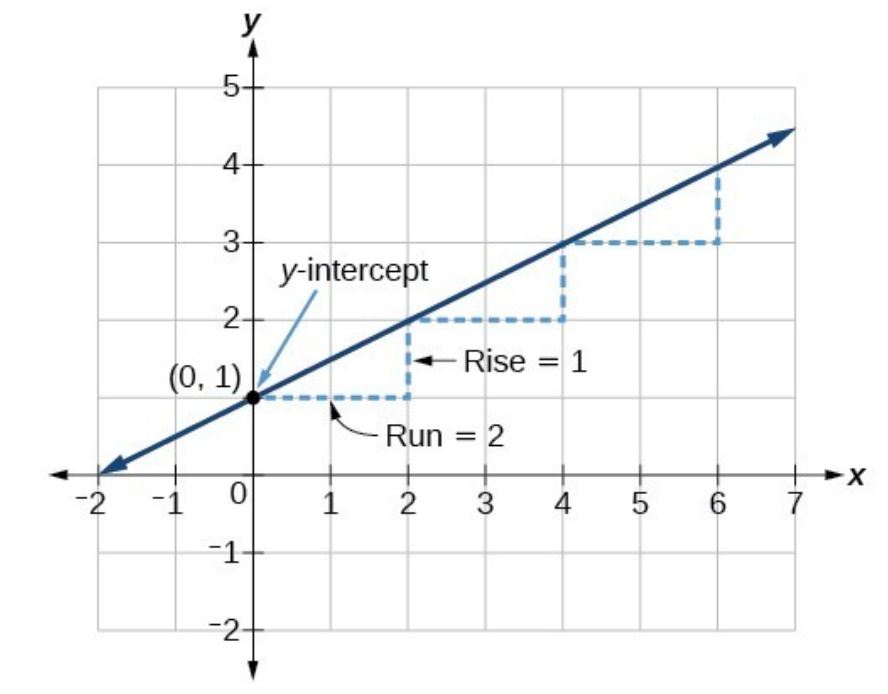
Example 4

Graph the following using information about the slope and the y-intercept: $y = \frac{1}{2} x + 1$

Solution

The slope is $\frac{1}{2}$ . Because the slope is positive, we know the graph will slant upward from left to right. The y-intercept is the point on the graph when $x = 0$ . The graph crosses the y-axis at $(0, 1)$ . Now we know the slope and the y-intercept.

We can begin graphing by plotting the point $(0, 1)$ . We also know that the slope is rise over run, $m = \frac{rise}{run}$ . We know the slope for our linear model is $\frac{1}{2}$ , which means that the rise is 1 and the run is 2. So starting from our y-intercept $(0, 1)$ , we can rise 1 and then run 2, or run 2 and then rise 1. We repeat until we have a few points, and then we draw a line through the points as shown below.

graph of the line y = (1/2)x +1 showing the rise, or change in the y direction as 1 and the run, or change in x direction as 2, and the y-intercept at (0,1)

Do all linear models have a y-intercept? What about x-intercept?

The general answer to this is no. Some linear models could be in the form of $x = c$ or $y = c$ , where c is some constant. The first linear equation when graphed forms a vertical line which the second is a horizontal line. Both of these, however, is not of interest to us as we are looking at the relationship between two variables that are related. For our work in this section we will only look at linear equations that do not represent a vertical or horizontal line.

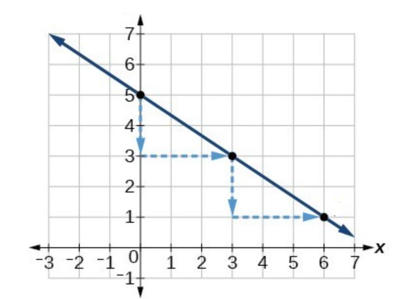
Try it Now 3

Graph the linear model by using information about the slope and y-intercept: $y = - \frac{2}{3} x + 5$

Hint 1

Start by identifying the slope and y-intercept. Recall for the form $y = m x + b$ we know m represents the slope and b the y-intercept.

Hint 2

The slope is $= \frac{2}{3}$ .

The y-intercept is 5, so we know the point $(0, 5)$ is on the line.

Answer

The slope is $= \frac{2}{3}$ and y-intercept is 5 giving us a point on the graph as $(0, 5)$ .

First thing to note is the slope is negative. This means as we look at the "rise" in the slope it will actually be a decrease. The slope tells us that for each movement in the horizontal direction "run" by 3 units the vertical direction "rise" will decrease by 2 units. We can now graph the linear model by first plotting the y-intercept. From the initial value $(0, 5)$ we move down 2 units and to the right 3 units. We can extend the line to the left and right by repeating, and then draw a line through the points.

graph of the line y = (-2/3)x + 5 showing the change of -2 in y and change of 3 in x.

Solve applications problems involving a linear model

We will keep our focus in this area related to our study of statistics in that we will be looking at how to construct a model from two given data points from a sample or a population of interest. In addition we will place emphasis on understanding the model in terms of the application presented.

When starting our work for finding a linear model between two quantitative variables in applications we will have to decide which variable is treated as x in the linear equation and which ones as y. If it is known that one variable is more dependent on the other variable we will assign that dependent variable as y and the other will be called the independent (or explanatory) variable and assigned to x. We will often, however, choose constants beyond x and y if those constants help keep track of what each variable represents in the application.

For instance if we are looking at the relationship between the age of a child and the number of words in the vocabulary we may want to use "a" for age and "v" for the number of words in the vocabulary. This use of "a" and "v" makes it easier to recognize how the model works instead of trying to figure out what the letters "x" and "y" represent.

Find a linear model in applications

Identify the variables in the given information.
Assign the variables letter names.
Identify if one variable is independent (or explanatory). If it is that variable is treated like x in our linear model. If there is no direct independent or dependent variable you can randomly assign which to be treated as x and which as y.
Write the given information as two ordered pairs.
Calculate the slope from the ordered pairs you constructed.
Find the y-intercept using the linear model with the slope you found above entered and one of the data points.
Put both the slope and y-intercept into the linear model.

Example 5

The number of words in a childs language is approximately linear when a child is between 12 months and 18 months (after about 18 months the growth in childrens vocabulary increases at a much faster rate). A particular childs vocabulary was tracked at age 12 months and age 18 months. At 12 months the vocabulary was 5 words and at age 18 months the vocabulary was 31 words. Create a linear model to show the relationship between number of words and age of a child.

Solution

To get started we should first identify the variables. We are given the age of a child and the number of words in the vocabulary. We will use the letter "a" to represent the age of the child and the letter "v" to represent the number of words in the vocabulary.

The age of a child best explains what we would see as a value for the number of words in the vocabulary. We will treat "a" as the x variable in the linear model and "v" as the y variable. This gives us our structure for the linear model as: $v = m a + b$

The information provide in the text gives us two data points in the form $(a, v)$ . At 12 months the child has a vocabulary of 5 words, so our first ordered pair is $(12, 5)$ . The second ordered pair would be $(18, 31)$ .

Calculate the slope: $m = \frac{(31 - 5)}{18 - 12} = \frac{26}{6} = \frac{13}{3}$

Using the information about the slope and the ordered pair $(12, 5)$ we can now find the y-intercept value:

\begin{array}{l} v = \frac{13}{3} a + b \\ 5 = \frac{13}{3} (12) + b \\ 5 = 13 (4) + b \\ 5 = 52 + b \\ 5 - 52 = b \\ - 47 = b \end{array}

The linear model that relates the age (in months), a, and the number of words in the vocabulary, v, is: $v = \frac{13}{3} a - 47$

We found a linear model that related the childs age in months to the number of words in their vocabulary. What does the value of slope mean for that application? The slope in the above example was $\frac{13}{3}$ . When the slope was calculated the values used represented:

slope = \frac{(change in number of words in vocabulary)}{(change in age)}

The slope was that change in number of words in the vocabulary over the change in age (in months). Putting this together with the value we have the interpretation of 13 words per 3 months. In other words we expect to see a gain of 13 words in the childs vocabulary for every three months of age.

What are the units of slope?

We have already looked at the formula for slope and saw it represents the $\frac{rise}{run}$ when viewing it graphically or as the $\frac{change in y}{change in x}$ is looking at the formula of the form $y = m x + b$ . In both situations what we have is the ratio of y values to x values. This means are units for slope will be the units of y over the units of x:

slope units = \frac{Units of y}{Units of x}

What about that y-intercept for our previous example? In this case the y-intercept would not meaning in the application as it would represent the number of words in the childs vocabulary at 0 months age. With what was told in the setup of the question a value of 0 for the age would not be okay to use for the linear model. In the next example we will examine the y-intercept in the application. In the work we will use $t = 0$ to represent the time in years from 2019.

Example 6

In the Fall of 2019 the PCC tuition for an in-state residents was $84.50 for 1 credit. In Fall of 2020 the tuition for an in-state resident was $87.00 for 1 credit. Construct a linear model for the cost of in-state resident tuition of 1 credit hour assuming the trend is linear and continues in that pattern.

What does the slope represent in our model?
What is the predicted tuition in 2024?
When would the tuition be over $150?

Solution

In this situation we have an independent variable of time (the years after 2019) and a dependent variable being the tuition cost as the year it is explains the cost in tuition we would see. Let t be the time (in years), but we will let $t = 0$ represent the year 2019. The dependent variable being tuition cost can be represented by c.

The data that was given to use can be written as a coordinate pair $(t, c)$ . In 2019 the cost for tuition was $84.50, so the corresponding ordered pair is $(0, 84.50)$ . In 2020 the tuition was $87.00 and gives the ordered pair as $(1, 87.00)$ .

Find the slope based on the data provided:

m = \frac{(87 - 84.50)}{1 - 0} = \frac{2.50}{1} = 2.50

In this instance we are given the y-intercept as we are using $t = 0$ to represent the tuition in 2019 with a value of &84.50. This means the value of b, the y-intercept, is 84.50 for the model.

Putting the slope and intercept into the model we have: $c = 2.50 t + 84.50$

Our interpretation for the slope is that the tuition will increase by $2.50 per year after 2019.

The y-intercept value of 84.50 is the starting tuition amount in 2019.
To find the tuition in 2024 we will evaluate the model at $t = 5$ as 2024 is fives years after 2019. $\begin{array}{l} c = 2.50 (5) + 84.50 \\ c = 12.50 + 84.50 \\ c = $ 97 \end{array}$
To find when the tuition is greater than $150 we can set the tuition in the model to 150 and solve for t. $\begin{array}{l} 150.00 = 2.50 t + 84.50 \\ 150.00 - 84.50 = 2.50 t \\ 65.50 = 2.50 t \\ \frac{65.50}{2.50} = t \\ 26.20 = t \end{array}$ The tuition reaches $150 a little after 26 years. If we use the model for $t = 26$ and $t = 27$ we see that it is over $150 when t=27 or the year 2046.

You may be asking why we wanted the start of the linear model in 2019 to be represented with $t = 0$ . The reason for this is to help with reading the model after it is created and having a better understanding of where the tuition started from by looking at the y-intercept value. When $t = 0$ the y-intercept is going to be $84.50; the starting tuition amount in 2019. If we had not picked that starting time as 2019 we would have ended up with a y-intercept that was negative and had not relation to the application for what happens when you enter 0 for the time (year).

Try it Now 4

The population of a small city was in 2012 was 32,500. By 2018 the city has grown to a population of 37,000. If we assume the population is growing with a linear trend, then find a linear model for the city's population and use the model to answer the following questions:

What does the slope mean in the model?
What would the predicted population be in 2021?
In what year would the population reach 45,000?

Answer

The two variables are the population and time. The time (year) explains how the population would change, so we will use time as our independent variable and the population as the dependent variable. Like the previous example we will let the time be represented by t, but be the number of years since 2012 (otherwise that y-intercept value would be a value for the population 2000 years ago and would have no meaning to us). The population can be represented with the letter p.

The given information gives us two ordered pairs as $(0, 32500) and (6, 37000)$ .

Calculate the slope:

\begin{array}{l} m = \frac{(37000 - 32500)}{6 - 0} \\ m = \frac{4500}{6} \\ m = 750 people per year \end{array}

By our choice for t being the time after 2012 we already know the value of the y-intercept as 32,500. Enter both the slope and y-intercept value to have the linear model: $p = 750 t + 32500$ .

Now that the linear model was found answer the given questions.

The slope represents the rate of change in the population to years. We found the slope to be equal to 750 and means the model is showing the population growing by 750 people each year.
To predict the population in 2021 we need to use $t = 9$ as 2021 is 9 years after 2012. $\begin{array}{l} p = 750 (9) + 32500 \\ p = 6, 750 + 32500 \\ p = 39, 250 \end{array}$ The population in 2021 would be 39,250 based on the model.
To find the year the population reaches 45,000 we will set $p = 45000$ and solve for t. $\begin{array}{l} 45000 = 750 t + 32500 \\ 45000 - 32500 = 750 t \\ 12500 = 750 t \\ \frac{12500}{750} = t \\ 16.67 \approx t \end{array}$ Our model predicts the population will reach 45,000 after 16.67 years from 2012. This would happen sometime in the year 2028.

Exercises

Identify which are linear models. If it is a linear model state the slope and y-intercept.
1. $y = - x + 10$
2. $y = 2^{x} - 5$
3. $y = \frac{4}{9} x - 1$
4. $y = 4 x^{3} + 2$
Answer
1. Linear: Slope is -1, y-intercept is 10
2. Not Linear
3. Linear: Slope is $\frac{4}{9}$ , y-intercept is -1
4. Not Linear
Find the equation of a line through the points $(2, 1) and (3, 5)$
Answer

$y = 4 x - 7$
Find the equation of a line through the points $(1, 3) and (5, 2)$
Answer

$y = - \frac{1}{4} x + \frac{13}{4}$
Find the equation of a line through $(- 3, - 2) and (0, 5)$
Answer

$y = \frac{7}{3} x + 5$
Graph the linear model given by $y = 5 x - 4$
Answer

Points picked will vary.

Graph of $y = 5 x - 4$ produced on Desmos. Go to Desmos to explore this model.
Graph the linear model given by $y = - x + 5$
Answer

Points picked will vary.

Graph of $y = - x + 5$ produced on Desmos. Go to Desmos to explore this model.
Graph the linear model given by $y = \frac{2}{3} x - 1$
Answer

Points picked will vary.

Graph of $y = \frac{2}{3} x - 1$ produced on Desmos. Go to Desmos to explore this model.
The population of beetles is assumed to be growing according to a linear model. The initial population was 30 beetles and after 8 weeks the population reached 62.
1. What is a linear model to represent the amount of beetles after t weeks?
2. How many beetles would we expect to find after 10 weeks?
3. In what week would we expect to see the population reach 150?
Answer
1. $P = 4 t + 30$
2. 70 beetles after 10 weeks. $\begin{array}{l} P = 4 (10) + 30 \\ P = 70 \end{array}$
3. In Week 30. $\begin{array}{l} 150 = 4 t + 30 \\ 120 = 4 t \\ 30 = t \end{array}$
The population of a town was 120,000 in 2010. In 2020 the town population was 180,000.
1. Write is a linear model to represent the population n years after 2010.
2. What does the model predict the population to be in 2025?
3. Based on the model when would the population reach 250,000?
Answer
ANSWER
1. $y = 6, 000 n + 120, 000$
2. 210,000 is the predicted population in 2025.
3. Based on the model the population would reach 250,000 during the year 2031. $\begin{array}{l} 250, 000 = 6, 000 n + 120, 000 \\ 130, 000 = 6, 000 n \\ \frac{130, 000}{6, 000} = n \\ 21.67 \approx n \end{array}$
A student tutors to help pay for college expenses. If they charge a flat fee of $20 plus $15 an hour, then we can model the total cost of money charges by the following: $y = 20 + 15 x$
Describe what the slope and intercept represent in the model.

Answer

The slope is 15 in the model. This represents the hourly rate of $15 per hour charged for tutoring.

The y-intercept is 20. This represents the flat fee charged for tutoring.
A Manufacturer believes there is a linear relationship between the number of widgets, n, they can sell and the price, p, it can charge for the widget. They have historical data that shows they can sell 7,000 widgets at a price of $10 per widget and 1,000 widgets at a price of $25 per widget. Find a linear model that relates the price and number of widgets that can be sold.
Answer

We will find the linear model in the form: $p = w n + b$
$\begin{array}{l} p = m n + b \\ m = \frac{(10 - 25)}{7000 - 1000} = \frac{- 15}{6000} = - \frac{1}{400} \\ p = - \frac{1}{400} n + b \\ 25 = - \frac{1}{400} (1000) + b \\ 25 = - \frac{5}{2} + b \\ 25 + \frac{5}{2} = b \\ \frac{55}{2} = b \\ p = - \frac{1}{400} n + \frac{55}{2} \end{array}$
An internet provider charges for service based on the model: $C = 10 + .15 n$ , where n is the number of GB of data used and C is the monthly charge in dollars. Interpret both the slope and y-intercept for the model in terms of the application.
Answer

The slope represents the rate of change. In the model there is a slope of 0.15 which would translated as $0.15 per GB of data used.

The y-intercept is an initial value where $n = 0$ . In the model the y-intercept is $10 which would mean that there is a flat $10 charge just for service without using any data.

This page contains modified content from David Lippman, "Math In Society, 2nd Edition." Licensed under CC BY-SA 4.0.
This page contains modified content from "College Algebra," Abramson, Jay et al., OpenStax. Licensed under CC BY 4.0.
This page contains content by Robert Foth, Math Faculty, Pima Community College, 2021. Licensed under CC BY 4.0.